Sourcepredict example2: Estimating source proportions
Preparing mixed samples
[1]:
import pandas as pd
from plotnine import *
import numpy as np
[2]:
cnt = pd.read_csv("../data/modern_gut_microbiomes_sources.csv", index_col=0)
labels = pd.read_csv("../data/modern_gut_microbiomes_labels.csv",index_col=0)
As in example 1, we’ll first split the dataset into training (95%) and testing(5%)
[3]:
cnt_train = cnt.sample(frac=0.95, axis=1)
cnt_test = cnt.drop(cnt_train.columns, axis=1)
train_labels = labels.loc[cnt_train.columns,:]
test_labels = labels.loc[cnt_test.columns,:]
[4]:
test_labels['labels'].value_counts()
[4]:
Homo_sapiens        11
Canis_familiaris     9
Soil                 2
Name: labels, dtype: int64
[5]:
cnt_test.head()
[5]:
| SRR061456 | SRR1175013 | SRR059395 | SRR1930141 | SRR1930247 | SRR1761710 | SRR1761700 | SRR7658605 | SRR7658665 | SRR7658625 | ... | ERR1916299 | ERR1914213 | ERR1915363 | ERR1913953 | ERR1913947 | ERR1916319 | ERR1915204 | ERR1914750 | mgm4477803_3 | mgm4477877_3 | |
|---|---|---|---|---|---|---|---|---|---|---|---|---|---|---|---|---|---|---|---|---|---|
| TAXID | |||||||||||||||||||||
| 0 | 14825759.0 | 4352892.0 | 13691926.0 | 27457943.0 | 1212101.0 | 24026729.0 | 18876667.0 | 7776902.0 | 34166674.0 | 15983447.0 | ... | 1481835.0 | 3254064.0 | 2182037.0 | 2225689.0 | 2292745.0 | 1549960.0 | 760058.0 | 1750182.0 | 5492333.0 | 6004642.0 |
| 6 | 0.0 | 0.0 | 107.0 | 193.0 | 0.0 | 87.0 | 94.0 | 0.0 | 215.0 | 105.0 | ... | 0.0 | 0.0 | 0.0 | 0.0 | 0.0 | 0.0 | 0.0 | 0.0 | 73.0 | 216.0 |
| 7 | 0.0 | 0.0 | 107.0 | 193.0 | 0.0 | 87.0 | 94.0 | 0.0 | 215.0 | 105.0 | ... | 0.0 | 0.0 | 0.0 | 0.0 | 0.0 | 0.0 | 0.0 | 0.0 | 73.0 | 216.0 |
| 9 | 96.0 | 101.0 | 70.0 | 412.0 | 0.0 | 395.0 | 199.0 | 299.0 | 563.0 | 369.0 | ... | 62.0 | 63.0 | 110.0 | 59.0 | 63.0 | 51.0 | 0.0 | 61.0 | 0.0 | 0.0 |
| 10 | 249.0 | 0.0 | 136.0 | 614.0 | 0.0 | 265.0 | 267.0 | 76.0 | 985.0 | 350.0 | ... | 66.0 | 174.0 | 0.0 | 74.0 | 73.0 | 62.0 | 0.0 | 66.0 | 0.0 | 0.0 |
5 rows × 22 columns
We then create a function to randomly select a sample from each source (dog as \(s_{dog}\) and human as \(s_{human}\)), and combine such as the new sample \(s_{mixed} = p1*s_{dog} + p1*s_{human}\)
[6]:
def create_mixed_sample(cnt, labels, p1, samp_name):
    rand_dog = labels.query('labels == "Canis_familiaris"').sample(1).index[0]
    rand_human = labels.query('labels == "Homo_sapiens"').sample(1).index[0]
    dog_samp = cnt[rand_dog]*p1
    human_samp = cnt[rand_human]*(1-p1)
    comb = dog_samp + human_samp
    comb = comb.rename(samp_name)
    meta = pd.DataFrame({'human_sample':[rand_human],'dog_sample':[rand_dog], 'human_prop':[(1-p1)], 'dog_prop':[p1]}, index=[samp_name])
    return(comb, meta)
We run this function for a range of mixed proportions (0 to 90%, by 10%), 3 time for each mix
[7]:
mixed_samp = []
mixed_meta = []
nb = 1
for i in range(3):
    for p1 in np.arange(0.1,1,0.1):
        s = create_mixed_sample(cnt=cnt_test, labels=test_labels, p1=p1, samp_name=f"mixed_sample_{nb}")
        mixed_samp.append(s[0])
        mixed_meta.append(s[1])
        nb += 1
[8]:
mixed_samples = pd.concat(mixed_samp, axis=1, keys=[s.name for s in mixed_samp]).astype(int)
mixed_samples.head()
[8]:
| mixed_sample_1 | mixed_sample_2 | mixed_sample_3 | mixed_sample_4 | mixed_sample_5 | mixed_sample_6 | mixed_sample_7 | mixed_sample_8 | mixed_sample_9 | mixed_sample_10 | ... | mixed_sample_18 | mixed_sample_19 | mixed_sample_20 | mixed_sample_21 | mixed_sample_22 | mixed_sample_23 | mixed_sample_24 | mixed_sample_25 | mixed_sample_26 | mixed_sample_27 | |
|---|---|---|---|---|---|---|---|---|---|---|---|---|---|---|---|---|---|---|---|---|---|
| TAXID | |||||||||||||||||||||
| 0 | 1320165 | 27791888 | 14189886 | 14720060 | 18710369 | 1414816 | 2910789 | 4518936 | 2282396 | 7217415 | ... | 5331330 | 24788154 | 2020394 | 5968886 | 3231719 | 10313424 | 8480642 | 5192549 | 5175478 | 4809264 |
| 6 | 0 | 172 | 65 | 52 | 107 | 0 | 0 | 21 | 10 | 0 | ... | 8 | 173 | 0 | 0 | 0 | 47 | 37 | 32 | 18 | 19 |
| 7 | 0 | 172 | 65 | 52 | 107 | 0 | 0 | 21 | 10 | 0 | ... | 8 | 173 | 0 | 0 | 0 | 47 | 37 | 32 | 18 | 19 |
| 9 | 6 | 463 | 158 | 237 | 313 | 30 | 74 | 61 | 36 | 280 | ... | 96 | 370 | 132 | 227 | 81 | 130 | 110 | 56 | 88 | 97 |
| 10 | 7 | 802 | 239 | 159 | 579 | 37 | 51 | 86 | 34 | 68 | ... | 183 | 552 | 113 | 73 | 24 | 166 | 144 | 84 | 106 | 127 |
5 rows × 27 columns
[9]:
mixed_metadata = pd.concat(mixed_meta)
mixed_metadata.head()
[9]:
| human_sample | dog_sample | human_prop | dog_prop | |
|---|---|---|---|---|
| mixed_sample_1 | SRR1930247 | ERR1913947 | 0.9 | 0.1 |
| mixed_sample_2 | SRR7658665 | ERR1913947 | 0.8 | 0.2 |
| mixed_sample_3 | SRR1761700 | ERR1914213 | 0.7 | 0.3 |
| mixed_sample_4 | SRR1761710 | ERR1915204 | 0.6 | 0.4 |
| mixed_sample_5 | SRR7658665 | ERR1914213 | 0.5 | 0.5 |
Now we can export the new “test” (sink) table to csv for sourcepredict
[10]:
mixed_samples.to_csv('mixed_samples_cnt.csv')
As well as the source count and labels table for the sources
[11]:
train_labels.to_csv('train_labels.csv')
cnt_train.to_csv('sources_cnt.csv')
Sourcepredict
For running Sourcepredict, we’ll change two parameters from their default values: - -me The default method used by Sourcepredict is T-SNE which a non-linear type of embedding, i.e. the distance between points doesn’t reflext their actual distance in the original dimensions, to achieve a better clustering, which is good for source prediction. Because here we’re more interested in source proportion estimation, rather than source prediction, we’ll choose a Multi Dimensional Scaling (MDS) which
is a type of linear embedding, where the distance between points in the lozer dimension match more the distances in the embedding in lower dimension, which is better for source proportion estimation. - -kne which is the number of neighbors in KNN algorithm: we use a greater (50) number of neighbors to reflect more global contribution of samples to the proportion estimation, instead of only the immediate neighbors. This will affect negatively the source prediction, but give better source
proportion estimations - -kw which is the weigth function in the KNN algorithm. By defaul a distance based weight function is apllied to give more weigth to closer samples. However, here, we’re more interested in source proportion estimation, rather than source prediction, so we’ll disregard the distance based weight function and give the same weight to all neighboring samples, regardless of their distance, with the uniform weight function.
[12]:
%%time
!python ../sourcepredict -s sources_cnt.csv \
               -l train_labels.csv \
               -n GMPR \
               -kne 50\
               -kw uniform \
               -me MDS \
               -e mixed_embedding.csv \
               -t 6 \
               mixed_samples_cnt.csv
Step 1: Checking for unknown proportion
  == Sample: mixed_sample_1 ==
        Adding unknown
        Normalizing (GMPR)
        Computing Bray-Curtis distance
        Performing MDS embedding in 2 dimensions
        KNN machine learning
        Training KNN classifier on 6 cores...
        -> Testing Accuracy: 1.0
        ----------------------
        - Sample: mixed_sample_1
                 known:98.48%
                 unknown:1.52%
  == Sample: mixed_sample_2 ==
        Adding unknown
        Normalizing (GMPR)
        Computing Bray-Curtis distance
        Performing MDS embedding in 2 dimensions
        KNN machine learning
        Training KNN classifier on 6 cores...
        -> Testing Accuracy: 0.99
        ----------------------
        - Sample: mixed_sample_2
                 known:99.73%
                 unknown:0.27%
  == Sample: mixed_sample_3 ==
        Adding unknown
        Normalizing (GMPR)
        Computing Bray-Curtis distance
        Performing MDS embedding in 2 dimensions
        KNN machine learning
        Training KNN classifier on 6 cores...
        -> Testing Accuracy: 1.0
        ----------------------
        - Sample: mixed_sample_3
                 known:98.79%
                 unknown:1.21%
  == Sample: mixed_sample_4 ==
        Adding unknown
        Normalizing (GMPR)
        Computing Bray-Curtis distance
        Performing MDS embedding in 2 dimensions
        KNN machine learning
        Training KNN classifier on 6 cores...
        -> Testing Accuracy: 1.0
        ----------------------
        - Sample: mixed_sample_4
                 known:98.8%
                 unknown:1.2%
  == Sample: mixed_sample_5 ==
        Adding unknown
        Normalizing (GMPR)
        Computing Bray-Curtis distance
        Performing MDS embedding in 2 dimensions
        KNN machine learning
        Training KNN classifier on 6 cores...
        -> Testing Accuracy: 1.0
        ----------------------
        - Sample: mixed_sample_5
                 known:98.82%
                 unknown:1.18%
  == Sample: mixed_sample_6 ==
        Adding unknown
        Normalizing (GMPR)
        Computing Bray-Curtis distance
        Performing MDS embedding in 2 dimensions
        KNN machine learning
        Training KNN classifier on 6 cores...
        -> Testing Accuracy: 1.0
        ----------------------
        - Sample: mixed_sample_6
                 known:98.48%
                 unknown:1.52%
  == Sample: mixed_sample_7 ==
        Adding unknown
        Normalizing (GMPR)
        Computing Bray-Curtis distance
        Performing MDS embedding in 2 dimensions
        KNN machine learning
        Training KNN classifier on 6 cores...
        -> Testing Accuracy: 1.0
        ----------------------
        - Sample: mixed_sample_7
                 known:98.48%
                 unknown:1.52%
  == Sample: mixed_sample_8 ==
        Adding unknown
        Normalizing (GMPR)
        Computing Bray-Curtis distance
        Performing MDS embedding in 2 dimensions
        KNN machine learning
        Training KNN classifier on 6 cores...
        -> Testing Accuracy: 1.0
        ----------------------
        - Sample: mixed_sample_8
                 known:98.48%
                 unknown:1.52%
  == Sample: mixed_sample_9 ==
        Adding unknown
        Normalizing (GMPR)
        Computing Bray-Curtis distance
        Performing MDS embedding in 2 dimensions
        KNN machine learning
        Training KNN classifier on 6 cores...
        -> Testing Accuracy: 1.0
        ----------------------
        - Sample: mixed_sample_9
                 known:98.48%
                 unknown:1.52%
  == Sample: mixed_sample_10 ==
        Adding unknown
        Normalizing (GMPR)
        Computing Bray-Curtis distance
        Performing MDS embedding in 2 dimensions
        KNN machine learning
        Training KNN classifier on 6 cores...
        -> Testing Accuracy: 1.0
        ----------------------
        - Sample: mixed_sample_10
                 known:98.48%
                 unknown:1.52%
  == Sample: mixed_sample_11 ==
        Adding unknown
        Normalizing (GMPR)
        Computing Bray-Curtis distance
        Performing MDS embedding in 2 dimensions
        KNN machine learning
        Training KNN classifier on 6 cores...
        -> Testing Accuracy: 0.99
        ----------------------
        - Sample: mixed_sample_11
                 known:99.16%
                 unknown:0.84%
  == Sample: mixed_sample_12 ==
        Adding unknown
        Normalizing (GMPR)
        Computing Bray-Curtis distance
        Performing MDS embedding in 2 dimensions
        KNN machine learning
        Training KNN classifier on 6 cores...
        -> Testing Accuracy: 1.0
        ----------------------
        - Sample: mixed_sample_12
                 known:98.5%
                 unknown:1.5%
  == Sample: mixed_sample_13 ==
        Adding unknown
        Normalizing (GMPR)
        Computing Bray-Curtis distance
        Performing MDS embedding in 2 dimensions
        KNN machine learning
        Training KNN classifier on 6 cores...
        -> Testing Accuracy: 1.0
        ----------------------
        - Sample: mixed_sample_13
                 known:98.48%
                 unknown:1.52%
  == Sample: mixed_sample_14 ==
        Adding unknown
        Normalizing (GMPR)
        Computing Bray-Curtis distance
        Performing MDS embedding in 2 dimensions
        KNN machine learning
        Training KNN classifier on 6 cores...
        -> Testing Accuracy: 1.0
        ----------------------
        - Sample: mixed_sample_14
                 known:98.48%
                 unknown:1.52%
  == Sample: mixed_sample_15 ==
        Adding unknown
        Normalizing (GMPR)
        Computing Bray-Curtis distance
        Performing MDS embedding in 2 dimensions
        KNN machine learning
        Training KNN classifier on 6 cores...
        -> Testing Accuracy: 1.0
        ----------------------
        - Sample: mixed_sample_15
                 known:98.49%
                 unknown:1.51%
  == Sample: mixed_sample_16 ==
        Adding unknown
        Normalizing (GMPR)
        Computing Bray-Curtis distance
        Performing MDS embedding in 2 dimensions
        KNN machine learning
        Training KNN classifier on 6 cores...
        -> Testing Accuracy: 1.0
        ----------------------
        - Sample: mixed_sample_16
                 known:98.48%
                 unknown:1.52%
  == Sample: mixed_sample_17 ==
        Adding unknown
        Normalizing (GMPR)
        Computing Bray-Curtis distance
        Performing MDS embedding in 2 dimensions
        KNN machine learning
        Training KNN classifier on 6 cores...
        -> Testing Accuracy: 1.0
        ----------------------
        - Sample: mixed_sample_17
                 known:98.48%
                 unknown:1.52%
  == Sample: mixed_sample_18 ==
        Adding unknown
        Normalizing (GMPR)
        Computing Bray-Curtis distance
        Performing MDS embedding in 2 dimensions
        KNN machine learning
        Training KNN classifier on 6 cores...
        -> Testing Accuracy: 1.0
        ----------------------
        - Sample: mixed_sample_18
                 known:98.48%
                 unknown:1.52%
  == Sample: mixed_sample_19 ==
        Adding unknown
        Normalizing (GMPR)
        Computing Bray-Curtis distance
        Performing MDS embedding in 2 dimensions
        KNN machine learning
        Training KNN classifier on 6 cores...
        -> Testing Accuracy: 0.9
        ----------------------
        - Sample: mixed_sample_19
                 known:99.79%
                 unknown:0.21%
  == Sample: mixed_sample_20 ==
        Adding unknown
        Normalizing (GMPR)
        Computing Bray-Curtis distance
        Performing MDS embedding in 2 dimensions
        KNN machine learning
        Training KNN classifier on 6 cores...
        -> Testing Accuracy: 1.0
        ----------------------
        - Sample: mixed_sample_20
                 known:98.48%
                 unknown:1.52%
  == Sample: mixed_sample_21 ==
        Adding unknown
        Normalizing (GMPR)
        Computing Bray-Curtis distance
        Performing MDS embedding in 2 dimensions
        KNN machine learning
        Training KNN classifier on 6 cores...
        -> Testing Accuracy: 1.0
        ----------------------
        - Sample: mixed_sample_21
                 known:98.48%
                 unknown:1.52%
  == Sample: mixed_sample_22 ==
        Adding unknown
        Normalizing (GMPR)
        Computing Bray-Curtis distance
        Performing MDS embedding in 2 dimensions
        KNN machine learning
        Training KNN classifier on 6 cores...
        -> Testing Accuracy: 1.0
        ----------------------
        - Sample: mixed_sample_22
                 known:98.48%
                 unknown:1.52%
  == Sample: mixed_sample_23 ==
        Adding unknown
        Normalizing (GMPR)
        Computing Bray-Curtis distance
        Performing MDS embedding in 2 dimensions
        KNN machine learning
        Training KNN classifier on 6 cores...
        -> Testing Accuracy: 1.0
        ----------------------
        - Sample: mixed_sample_23
                 known:98.48%
                 unknown:1.52%
  == Sample: mixed_sample_24 ==
        Adding unknown
        Normalizing (GMPR)
        Computing Bray-Curtis distance
        Performing MDS embedding in 2 dimensions
        KNN machine learning
        Training KNN classifier on 6 cores...
        -> Testing Accuracy: 1.0
        ----------------------
        - Sample: mixed_sample_24
                 known:98.48%
                 unknown:1.52%
  == Sample: mixed_sample_25 ==
        Adding unknown
        Normalizing (GMPR)
        Computing Bray-Curtis distance
        Performing MDS embedding in 2 dimensions
        KNN machine learning
        Training KNN classifier on 6 cores...
        -> Testing Accuracy: 1.0
        ----------------------
        - Sample: mixed_sample_25
                 known:98.48%
                 unknown:1.52%
  == Sample: mixed_sample_26 ==
        Adding unknown
        Normalizing (GMPR)
        Computing Bray-Curtis distance
        Performing MDS embedding in 2 dimensions
        KNN machine learning
        Training KNN classifier on 6 cores...
        -> Testing Accuracy: 1.0
        ----------------------
        - Sample: mixed_sample_26
                 known:98.48%
                 unknown:1.52%
  == Sample: mixed_sample_27 ==
        Adding unknown
        Normalizing (GMPR)
        Computing Bray-Curtis distance
        Performing MDS embedding in 2 dimensions
        KNN machine learning
        Training KNN classifier on 6 cores...
        -> Testing Accuracy: 1.0
        ----------------------
        - Sample: mixed_sample_27
                 known:98.48%
                 unknown:1.52%
Step 2: Checking for source proportion
        Computing weighted_unifrac distance on species rank
        MDS embedding in 2 dimensions
        KNN machine learning
        Trained KNN classifier with 50 neighbors
        -> Testing Accuracy: 0.88
        ----------------------
        - Sample: mixed_sample_1
                 Canis_familiaris:87.65%
                 Homo_sapiens:11.14%
                 Soil:1.21%
        - Sample: mixed_sample_2
                 Canis_familiaris:3.66%
                 Homo_sapiens:95.03%
                 Soil:1.31%
        - Sample: mixed_sample_3
                 Canis_familiaris:3.66%
                 Homo_sapiens:95.03%
                 Soil:1.31%
        - Sample: mixed_sample_4
                 Canis_familiaris:5.65%
                 Homo_sapiens:93.02%
                 Soil:1.33%
        - Sample: mixed_sample_5
                 Canis_familiaris:3.66%
                 Homo_sapiens:95.03%
                 Soil:1.31%
        - Sample: mixed_sample_6
                 Canis_familiaris:92.78%
                 Homo_sapiens:6.02%
                 Soil:1.2%
        - Sample: mixed_sample_7
                 Canis_familiaris:54.39%
                 Homo_sapiens:44.26%
                 Soil:1.35%
        - Sample: mixed_sample_8
                 Canis_familiaris:36.94%
                 Homo_sapiens:61.66%
                 Soil:1.4%
        - Sample: mixed_sample_9
                 Canis_familiaris:5.65%
                 Homo_sapiens:93.02%
                 Soil:1.33%
        - Sample: mixed_sample_10
                 Canis_familiaris:5.65%
                 Homo_sapiens:93.02%
                 Soil:1.33%
        - Sample: mixed_sample_11
                 Canis_familiaris:5.65%
                 Homo_sapiens:93.02%
                 Soil:1.33%
        - Sample: mixed_sample_12
                 Canis_familiaris:30.32%
                 Homo_sapiens:68.27%
                 Soil:1.41%
        - Sample: mixed_sample_13
                 Canis_familiaris:5.65%
                 Homo_sapiens:93.02%
                 Soil:1.33%
        - Sample: mixed_sample_14
                 Canis_familiaris:30.32%
                 Homo_sapiens:68.27%
                 Soil:1.41%
        - Sample: mixed_sample_15
                 Canis_familiaris:24.34%
                 Homo_sapiens:74.24%
                 Soil:1.41%
        - Sample: mixed_sample_16
                 Canis_familiaris:30.32%
                 Homo_sapiens:68.27%
                 Soil:1.41%
        - Sample: mixed_sample_17
                 Canis_familiaris:27.24%
                 Homo_sapiens:71.35%
                 Soil:1.41%
        - Sample: mixed_sample_18
                 Canis_familiaris:83.76%
                 Homo_sapiens:15.02%
                 Soil:1.22%
        - Sample: mixed_sample_19
                 Canis_familiaris:24.34%
                 Homo_sapiens:74.24%
                 Soil:1.41%
        - Sample: mixed_sample_20
                 Canis_familiaris:3.66%
                 Homo_sapiens:95.03%
                 Soil:1.31%
        - Sample: mixed_sample_21
                 Canis_familiaris:5.65%
                 Homo_sapiens:93.02%
                 Soil:1.33%
        - Sample: mixed_sample_22
                 Canis_familiaris:40.4%
                 Homo_sapiens:58.2%
                 Soil:1.4%
        - Sample: mixed_sample_23
                 Canis_familiaris:3.66%
                 Homo_sapiens:95.03%
                 Soil:1.31%
        - Sample: mixed_sample_24
                 Canis_familiaris:3.66%
                 Homo_sapiens:95.03%
                 Soil:1.31%
        - Sample: mixed_sample_25
                 Canis_familiaris:30.32%
                 Homo_sapiens:68.27%
                 Soil:1.41%
        - Sample: mixed_sample_26
                 Canis_familiaris:21.65%
                 Homo_sapiens:76.94%
                 Soil:1.41%
        - Sample: mixed_sample_27
                 Canis_familiaris:85.18%
                 Homo_sapiens:13.6%
                 Soil:1.22%
Sourcepredict result written to mixed_samples_cnt.sourcepredict.csv
Embedding coordinates written to mixed_embedding.csv
CPU times: user 4.84 s, sys: 1.13 s, total: 5.97 s
Wall time: 5min 14s
Reading Sourcepredict results
[13]:
sp_ebd = pd.read_csv("mixed_embedding.csv", index_col=0)
[14]:
sp_ebd.head()
[14]:
| PC1 | PC2 | labels | name | |
|---|---|---|---|---|
| SRR1761712 | -3.713176 | -0.344326 | Homo_sapiens | SRR1761712 |
| ERR1913614 | 2.586560 | -0.498098 | Canis_familiaris | ERR1913614 |
| ERR1914349 | -1.595982 | -3.363762 | Canis_familiaris | ERR1914349 |
| SRR1930255 | 2.174966 | -0.728862 | Homo_sapiens | SRR1930255 |
| SRR1646027 | -3.329213 | -0.214682 | Homo_sapiens | SRR1646027 |
[15]:
import warnings
warnings.filterwarnings('ignore')
[16]:
ggplot(data = sp_ebd, mapping = aes(x='PC1',y='PC2')) + geom_point(aes(color='labels')) + theme_classic()
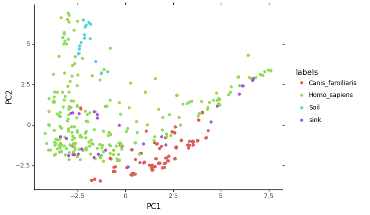
[16]:
<ggplot: (-9223372029299469603)>
[17]:
sp_pred = pd.read_csv("mixed_samples_cnt.sourcepredict.csv", index_col=0)
[18]:
sp_pred.T.head()
[18]:
| Canis_familiaris | Homo_sapiens | Soil | unknown | |
|---|---|---|---|---|
| mixed_sample_1 | 0.863266 | 0.109678 | 0.011905 | 0.015152 |
| mixed_sample_2 | 0.036542 | 0.947680 | 0.013046 | 0.002733 |
| mixed_sample_3 | 0.036198 | 0.938776 | 0.012923 | 0.012103 |
| mixed_sample_4 | 0.055810 | 0.919077 | 0.013163 | 0.011951 |
| mixed_sample_5 | 0.036211 | 0.939098 | 0.012927 | 0.011764 |
[19]:
mixed_metadata.head()
[19]:
| human_sample | dog_sample | human_prop | dog_prop | |
|---|---|---|---|---|
| mixed_sample_1 | SRR1930247 | ERR1913947 | 0.9 | 0.1 |
| mixed_sample_2 | SRR7658665 | ERR1913947 | 0.8 | 0.2 |
| mixed_sample_3 | SRR1761700 | ERR1914213 | 0.7 | 0.3 |
| mixed_sample_4 | SRR1761710 | ERR1915204 | 0.6 | 0.4 |
| mixed_sample_5 | SRR7658665 | ERR1914213 | 0.5 | 0.5 |
[20]:
sp_res = sp_pred.T.merge(mixed_metadata, left_index=True, right_index=True)
[21]:
sp_res.head()
[21]:
| Canis_familiaris | Homo_sapiens | Soil | unknown | human_sample | dog_sample | human_prop | dog_prop | |
|---|---|---|---|---|---|---|---|---|
| mixed_sample_1 | 0.863266 | 0.109678 | 0.011905 | 0.015152 | SRR1930247 | ERR1913947 | 0.9 | 0.1 |
| mixed_sample_2 | 0.036542 | 0.947680 | 0.013046 | 0.002733 | SRR7658665 | ERR1913947 | 0.8 | 0.2 |
| mixed_sample_3 | 0.036198 | 0.938776 | 0.012923 | 0.012103 | SRR1761700 | ERR1914213 | 0.7 | 0.3 |
| mixed_sample_4 | 0.055810 | 0.919077 | 0.013163 | 0.011951 | SRR1761710 | ERR1915204 | 0.6 | 0.4 |
| mixed_sample_5 | 0.036211 | 0.939098 | 0.012927 | 0.011764 | SRR7658665 | ERR1914213 | 0.5 | 0.5 |
[22]:
from sklearn.metrics import r2_score, mean_squared_error
[23]:
mse_sp = round(mean_squared_error(y_pred=sp_res['Homo_sapiens'], y_true=sp_res['human_prop']),2)
[24]:
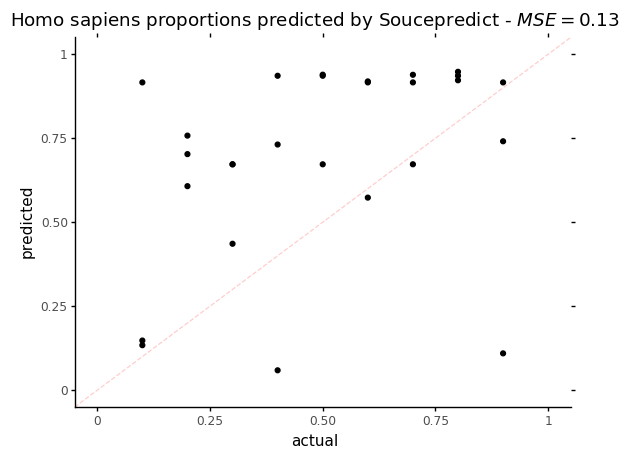
p = ggplot(data = sp_res, mapping=aes(x='human_prop',y='Homo_sapiens')) + geom_point()
p += labs(title = f"Homo sapiens proportions predicted by Soucepredict - $MSE = {mse_sp}$", x='actual', y='predicted')
p += theme_classic()
p += coord_cartesian(xlim=[0,1], ylim=[0,1])
p += geom_abline(intercept=0, slope=1, color = "red", alpha=0.2, linetype = 'dashed')
p
[24]:
<ggplot: (-9223372036555534967)>
On this plot, the dotted red line represents what a perfect proportion estimation would give, with a Mean Squared Error (MSE) = 0.
[25]:
sp_res_hist = (sp_res['human_prop'].append(sp_res['Homo_sapiens']).to_frame(name='Homo_sapiens_prop'))
sp_res_hist['source'] = (['actual']*sp_res.shape[0]+['predicted']*sp_res.shape[0])
[47]:
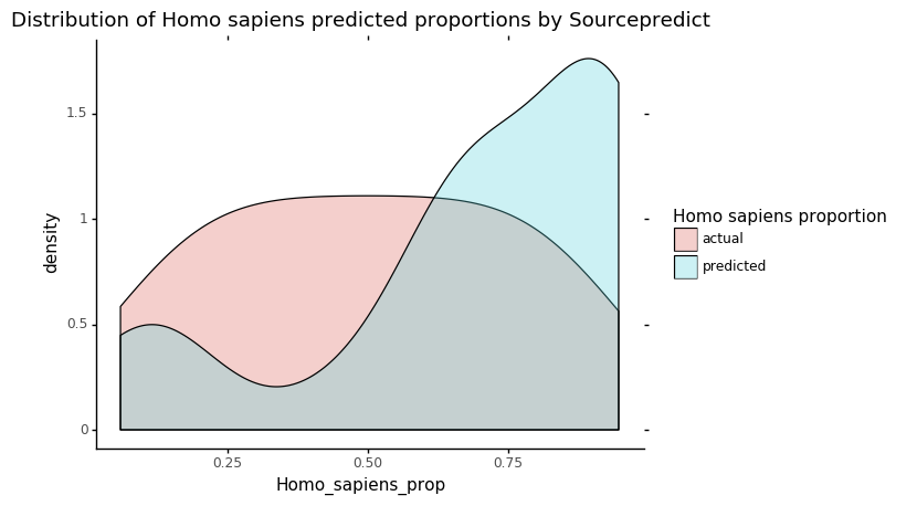
p = ggplot(data = sp_res_hist, mapping=aes(x='Homo_sapiens_prop')) + geom_density(aes(fill='source'), alpha=0.3)
p += labs(title = 'Distribution of Homo sapiens predicted proportions by Sourcepredict')
p += scale_fill_discrete(name="Homo sapiens proportion")
p += theme_classic()
p
[47]:
<ggplot: (-9223372029298930965)>
This plot shows the actual and predicted by Sourcepredict distribution of Human proportions. What we are interested in is the overlap between the two colors: the higer it is, the more the estimated Human proportion is accurate.
Sourcetracker2
Preparing count table
[27]:
cnt_train.merge(mixed_samples, right_index=True, left_index=True).to_csv("st_mixed_count.csv" , sep="\t", index_label="TAXID")
[28]:
!biom convert -i st_mixed_count.csv -o st_mixed_count.biom --table-type="Taxon table" --to-json
Preparing metadata
[29]:
train_labels['SourceSink'] = ['source']*train_labels.shape[0]
[30]:
mixed_metadata['labels'] = ['-']*mixed_metadata.shape[0]
mixed_metadata['SourceSink'] = ['sink']*mixed_metadata.shape[0]
[31]:
st_labels = train_labels.append(mixed_metadata[['labels', 'SourceSink']])
[32]:
st_labels = st_labels.rename(columns={'labels':'Env'})[['SourceSink','Env']]
[33]:
st_labels.to_csv("st_mixed_labels.csv", sep="\t", index_label='#SampleID')
sourcetracker2 gibbs -i st_mixed_count.biom -m st_mixed_labels.csv -o mixed_prop --jobs 6Sourcetracker2 results
[40]:
st_pred = pd.read_csv("mixed_prop/mixing_proportions.txt", sep="\t", index_col=0)
[41]:
st_res = st_pred.merge(mixed_metadata, left_index=True, right_index=True)
[42]:
mse_st = round(mean_squared_error(y_pred=st_res['Homo_sapiens'], y_true=st_res['human_prop']),2)
[43]:
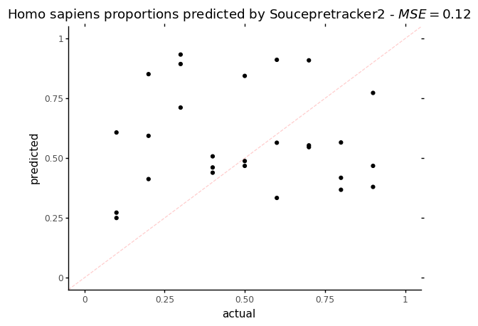
p = ggplot(data = st_res, mapping=aes(x='human_prop',y='Homo_sapiens')) + geom_point()
p += labs(title = f"Homo sapiens proportions predicted by Soucepretracker2 - $MSE = {mse_st}$", x='actual', y='predicted')
p += theme_classic()
p += coord_cartesian(xlim=[0,1], ylim=[0,1])
p += geom_abline(intercept=0, slope=1, color = "red", alpha=0.2, linetype = 'dashed')
p
[43]:
<ggplot: (-9223372029300899661)>
On this plot, the dotted red line represents what a perfect proportion estimation would give, with a Mean Squared Error (MSE) = 0. Regarding the MSE, Sourcepredict and Sourcetracker perform similarly with a MSE of 0.13 for Sourcepredict and 0.12 for Sourcetracker.
[44]:
st_res_hist = (st_res['human_prop'].append(st_res['Homo_sapiens']).to_frame(name='Homo_sapiens_prop'))
st_res_hist['source'] = (['actual']*st_res.shape[0]+['predicted']*st_res.shape[0])
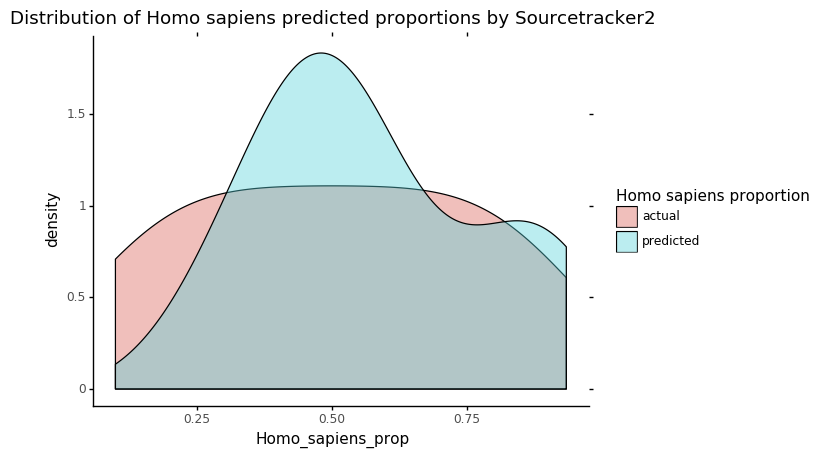
[46]:
p = ggplot(data = st_res_hist, mapping=aes(x='Homo_sapiens_prop')) + geom_density(aes(fill='source'), alpha=0.4)
p += labs(title = 'Distribution of Homo sapiens predicted proportions by Sourcetracker2')
p += scale_fill_discrete(name="Homo sapiens proportion")
p += theme_classic()
p
[46]:
<ggplot: (7555587890)>